Blueprint 3: "Divide and Conquer" ⚔️
Blueprint 3: Divide and Conquer ⚔️
Welcome, Architect. So far, our tools have been powerful but direct. To build truly legendary structures, we must move beyond brute force. Today, we learn a strategy of elegance and efficiency, a principle that turns overwhelming challenges into manageable tasks: Divide and Conquer.
1. The Mission Briefing
The brute-force sorting protocol, with its O(n²) complexity, is like trying to build a skyscraper one pebble at a time. It's inefficient, slow, and scales poorly. Master architects don't work harder; they work smarter. They use Divide and Conquer.
The principle is simple yet profound: if a problem is too big and scary, break it into smaller, identical subproblems. Keep breaking them down until they become so small that the solution is obvious. Then, skillfully combine the solutions to those small problems to solve the original grand challenge.
2. The Analogy: Sorting a Deck of Cards
Imagine you're handed a shuffled deck of 52 cards and told to sort it. Trying to manage all 52 cards at once, finding the right place for each, is a complex mental task.
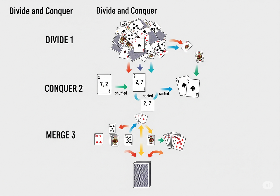
Let's apply Divide and Conquer:
- Divide: Split the deck of 52 cards in half. Now you have two piles of 26. This is still too complex. Split those piles. Keep splitting until you have 52 individual piles, each with only one card.
- Conquer: How do you sort a pile of one card? You don't! A single card is already sorted. This is our base case—the problem that's so simple, its solution is trivial.
- Combine: Now, merge the 1-card piles back together into sorted 2-card piles. Then merge those into sorted 4-card piles, and so on. At each step, you are merging two already sorted piles, which is a much simpler task. You continue this process until you have one single, perfectly sorted deck of 52 cards.
This exact strategy is the foundation of an algorithm called Merge Sort, which we will explore in detail.
Deep Dive: The Engine of Recursion
The Divide and Conquer strategy is most naturally implemented using a powerful programming concept called recursion.
The Logic: A Chain of Command
Think of recursion as a general giving a command to a chain of command. The General is given the big problem: "Sort this pile of 52 cards!". The General can't do it alone. So, they split the pile in two and tell two Colonels: "Each of you, sort these smaller piles of 26."
The Colonels can't do it either. They split their piles and command their Majors. This continues down the ranks—Captain, Lieutenant—until a Second Lieutenant is handed a pile with just one or two cards. They can easily sort this tiny pile (the base case). Once sorted, the Lieutenant reports back to their Captain with a sorted pile. The Captain merges the two piles they received from their Lieutenants and reports the now-larger sorted pile up to the Major. This merging process continues up the chain of command until the General receives the final, fully sorted deck. A recursive function works the same way: it calls itself on smaller inputs until it hits a simple base case, and then the solution is passed back up the chain of calls.
The Anatomy of a Recursive Function
Every well-formed recursive function has two essential parts:
- The Base Case: This is the stopping condition. It's a simple version of the problem that the function can solve directly without calling itself again. A function without a proper base case will call itself forever, leading to an error.
- The Recursive Step: This is where the function does two things:
- It breaks the current problem down into a slightly smaller version.
- It calls itself on that smaller problem.
Let's see this in action with a classic example: calculating a factorial. The factorial of a number n, denoted n!, is the product of all positive integers up to n (e.g., 4! = 4 * 3 * 2 * 1 = 24).
def factorial(n):
    # Base Case: The factorial of 0 is 1.
    if n == 0:
        return 1
    # Recursive Step: n! = n * (n-1)!
    else:
        return n * factorial(n - 1)
How Recursion Actually Works: The Call Stack
How does the computer keep track of all these function calls? It uses a data structure called the Call Stack. Think of it as a stack of plates. Each time a function is called, a new "plate" (a stack frame) containing that function's details (its parameters, local variables) is placed on top of the stack. When a function finishes and returns a value, its plate is removed from the top.
The Recursive Call Stack: factorial(3)
Visualize how the call stack manages recursive function calls. Each call adds a "frame" to the stack.
Call Stack is Empty
Press Start to visualize.
Recursion vs. Iteration
Every recursive algorithm can also be written iteratively (using loops like for or while). So why choose one over the other?
- Recursion Pros: Can lead to cleaner, more readable, and more elegant code, especially for problems that are naturally recursive, like tree traversals or Divide and Conquer.
- Recursion Cons: Can be less efficient. Each function call adds overhead and consumes memory on the call stack. If the recursion is too deep, you can get a Stack Overflow Error.
- Iteration Pros: Generally faster and uses less memory as it doesn't add new frames to the call stack. Avoids any risk of stack overflow.
- Iteration Cons: For complex recursive problems, the iterative solution can be much harder to write and understand. It may require you to manage your own stack data structure explicitly.
The Divide and Conquer Blueprint
Now that we understand recursion, let's formalize the three steps of the Divide and Conquer paradigm.
- Divide: Break the input problem of size n into a smaller subproblems, each of size n/b.
- Conquer: Solve the a subproblems recursively. If the subproblem size is small enough (the base case), solve it directly.
- Combine: Take the solutions from the subproblems and combine them into a solution for the original problem. This step's complexity is crucial.
Analyzing D&C Algorithms: Recurrence Relations
We can precisely describe the runtime of a D&C algorithm using a recurrence relation. This is just an equation that defines a function in terms of itself.
For our card sorting (Merge Sort) example: T(n) = 2T(n/2) + O(n).
- T(n): The total time to solve a problem of size n.
- 2T(n/2): The time it takes to solve two subproblems (a=2) that are half the size (b=2) of the original. This is the recursive "Conquer" part.
- O(n): The time it takes to do the work of splitting the piles and, more importantly, merging the sorted halves back together. This is the "Combine" step.
For a comprehensive course, the Master Theorem is a tool that acts as a "cheat code" to solve many common recurrence relations like this one, allowing us to quickly find the Big O complexity without complex math.
Core D&C Algorithms in Action
Algorithm 1: Merge Sort
This is the direct implementation of our card sorting analogy. Its brilliance lies in the merge step, which is highly efficient.
- Divide: Split the array in half until you have arrays of size 1.
- Conquer: An array of size 1 is already sorted.
- Combine: Repeatedly merge the sorted subarrays. The merge function takes two sorted arrays and combines them into a single sorted array in linear time, O(n).
Merge Sort Visualization
An animated look at how this algorithm operates.
Analysis: Merge Sort has a consistent and reliable time complexity of O(n log n) in all cases (worst, average, and best). Its main drawback is that it requires extra space, O(n), for the merged arrays.
Algorithm 2: Quick Sort
Quick Sort is another brilliant D&C sorting algorithm, but it flips the script. The hard work is done in the "Divide" step, making the "Combine" step trivial.
- Divide: Choose an element from the array, called the pivot. Rearrange the array so that all elements smaller than the pivot are to its left, and all elements larger are to its right. This is called partitioning. The pivot is now in its final sorted position.
- Conquer: Recursively apply Quick Sort to the subarray of smaller elements and the subarray of larger elements.
- Combine: Nothing! Because the pivot is already in its correct place and the subarrays will be sorted in place, no merging is needed.
The choice of pivot is critical. A good pivot splits the array into roughly equal halves. A bad pivot (e.g., the smallest or largest element) can degrade performance significantly.
Quick Sort Visualization
An animated look at how this algorithm operates.
Analysis: Best/Average Case: O(n log n). Worst Case: O(n²).
Despite its worst-case potential, Quick Sort is often faster in practice than Merge Sort because it operates in-place and has better cache performance.
Algorithm 3: Binary Search
Binary Search is the quintessential example of a D&C algorithm applied to searching, not sorting. It's how you find a word in a dictionary or a name in a phone book. Prerequisite: The array must be sorted.
- Divide: Compare the target value with the middle element of the array. This divides the search space in half.
- Conquer:
- If the middle element is the target, you've found it!
- If the target is smaller, recursively search in the left half.
- If the target is larger, recursively search in the right half.
- Combine: Trivial. No work is needed. The result of the recursive call is the final result.
Analysis: With each step, you cut the search space in half. This gives Binary Search a highly efficient logarithmic time complexity of O(log n).
Interactive Binary Search
Visualize how binary search efficiently finds a target in a sorted array.
Enter a number and click search.